Recently, I needed a robust way to calculate the curvature for a cubic bezier curve. Now there are plenty of guides on how to do this, but when I implemented the usual methods I got some weird results.

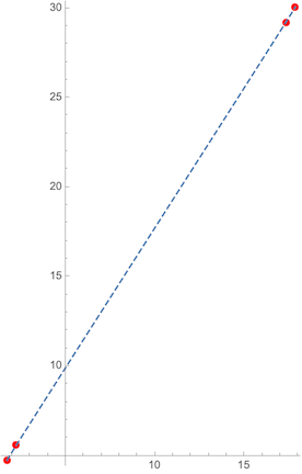
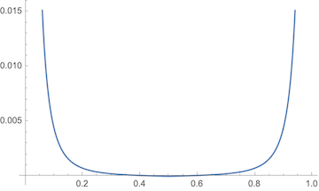
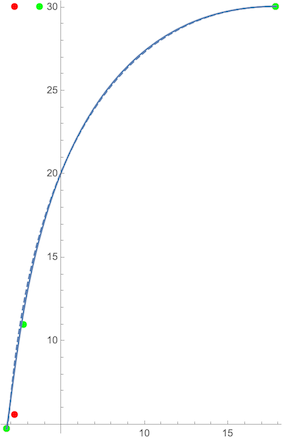
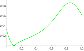
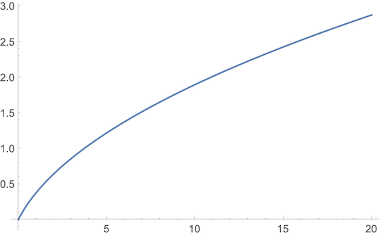
Here is, I think we can agree, what seems like a straight line, with the cubic control points marked. When we calculate the curvature however we get something a bit weird:

At first I thought I had implemented this wrong. (It's correct.) Then I started to wonder if maybe the "curvature of a line" is a silly notion and I should special-case it in my code. That's when I found this:

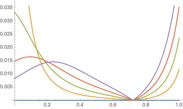
The meaning of these charts are that the curvature of the cubic is strongest at the origin. But if you imagine yourself traveling along the cubic like an arc, it doesn't "feel" like you're turning sharply at the origin. It "feels" like you're turning sharply about 3/4 of the way along. And indeed, the curvature graph has that too as a local maxima; it's just dwarfed by the curvature at the very beginning.

A discontinuity

It turns out that the curvature formula has a very nasty discontinuity. To see this, let's look at the formula:

It's clear something bad can happen if the denominator gets very small. Now we can expand this out in control point notation easily enough, but it's a nasty denominator that doesn't really have an obvious meaning to me. So, let's convert to another notation recommended by a friend instead:

• $r$ - the distance between the endpoints
• $tt$ the direction of a vector between the endpoints
• $tt_{0}$ The difference between the initial tangent angle and $tt$. (For a control point on the line between endpoints, the tangent angle is $tt$, and so $tt_{0} = 0$.)
• $tt_{1}$ - Like $tt_{0}$ but for the final tangent angle.
• $r_{0}, r_{1}$ the length of initial and final tangent vectors

In this notation a cubic is parameterized with

What do we gain with this notation? One advantage is that at $t=0$, the curvature equation has an "easy" solution:

Therefore, the curvature will be infinite with $\lim\limits_{r_{0} \to 0}$, e.g. as the control point gets closer to the endpoint.

So, make sure your control points and endpoints aren't the same and they won't have zero distance and you don't divide by zero. Not so tough, right?

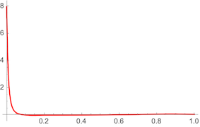
Turns out it's a little more complicated than that. Let's consider what happens when $r_{0}$ is a perfectly reasonable number like 20:

Here, we might expect that $r_{0}=0$ is not curved, $r_{0}=20$ is a little bit curved, and so on, with $r_{0}=80$ being the most curved. However, when we crunch the numbers:

It's true as long as you check at $t>0.2$ or so. But if you judge the lines by their greatest curvature, it's at the endpoints. $r_{0}=20$ is the most curved, followed by $r_{0}=40$, $r_{0}=60$, $r_{0}=80$, and finally $r_{0}=0$. Other than the last one, this is the complete opposite of what I expected. It's as if you're trying to draw a straight line, and the harder you try, the more curved it is. (Unless you nail it, then it's fine.)

The problem is not really the undefined behavior when $r_{0}=0$, the problem is the well-defined division when it isn't.

Papering over the problem

I am a bit surprised that I can't google up some prior art on how to deal with this. I did find one stackexchange answer suggesting such curves are not "regular", but "this is unlikely to happen", and googling that terminology didn't help.

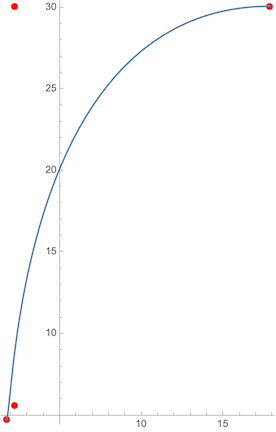
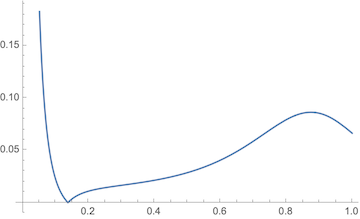
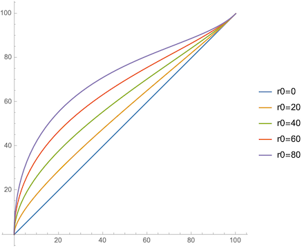
I did notice just playing around that I can make a "similar" cubic with larger $r_{0}$ that has nice curvature:

This suggests that I can pick a new control point for a larger $r_{0},r_{1}$ and get a nice curvature that way.

Picking $r_{0}$

There is some prior art on this general topic. For example, I found this paper which says

A reason for one to get undesired shapes is unsuitable magnitudes of the given tangent vectors. Usually, the larger the magnitudes of the tangent vectors, the more likely the occurrence of a loop in the resulting curve. On the other hand, the smaller the magnitudes of the tangent vectors, the closer the resulting curve to the base line segment. Therefore, the problem is how to choose suitable magnitudes for the endpoint tangent vectors.

That sounds very promising. Unfortunately, their solution is not overly interested in a nice curvature and it also involves assembling multiple cubics into a megazord cubic ("composite optimized geometric Hermite cubic" for short) and then using that, which is not ideal for my case.

Instead, I noticed that if we take the curvature equation from earlier, and let $t=0, r_{1}=r_{0}, tt_{0}=+err, tt_{1}=-err$ we get

The idea here is that we have a line that is "nearly straight" (curved a little by $err$), and then we hold the resulting curvature below some $k$:

Now we just pick an $err$ that seems straight (a few degrees), a $k$ that seems small ($0.02$), and crank out an $r_{0}$:

Here we see that I wanted $r_{0}$ to be at least 3, but in many of my examples it's only 1. Bumping it up makes the curvature nice again.

A few observations about this formula

If you want the "smallest possible" $k$ to address this problem, the practical limit of this expression in $\lim\limits_{k \to 0}$ seems to be $r_{0} == {r\over2}$. I say the "practical limit" because, well, if $k$ gets very small, things get a little odd:

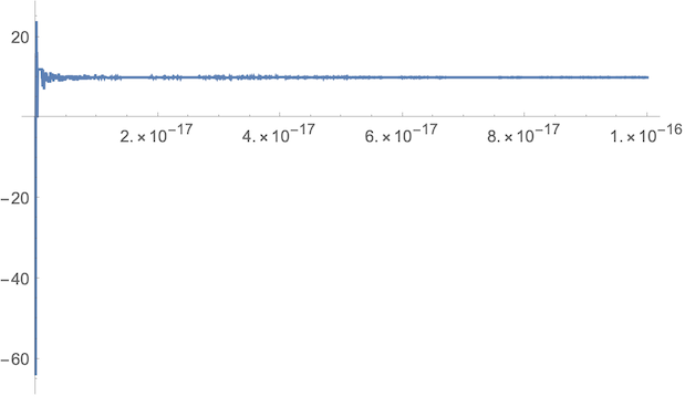
So the analytical limit looks indeterminate. Still, the $r\over2$ rule works well enough for many graphical applications.

However, $r\over2$ may be overly large if you can tolerate some asymptotic behavior. For example, if you're implementing the curvature, and want to know if you can do something reasonable for a given input curve, the full form may be more useful.

An implementation of this function appears in blitcurve, my general-purpose bezier geometry library.

Applying $r_{0}$

So if this how we get the $r_{0},$ what do we do with it? In the case of the line it is pretty easy; any control point along the line will produce "the same" line, so we just pick control points along the line with a new $r_{0}$ and we're done.

In general, however, a cubic with moved control points will be a different path. This situation was not important to my immediate problem, so I did not look into it extensively. However, I believe it can be done by reparameterizing to control-point notation and solving for the missing points.